27. SDR Frameworks

When you want to build an SDR or RF signal processing application, you must choose whether to write it as a bespoke application from scratch, or whether it’s worth using an existing SDR framework. In most SDR frameworks, you connect pre-built processing blocks together (often with some of your own custom blocks) and a runtime handles moving samples between them. The SDR framework tends to also come with GUIs and signal debugging tools, and sometimes support for a variety of hardware. By creating an application within this type of framework, you automatically get support for many SDRs and you don’t have to spend as much time writing GUIs and such. In this chapter we will learn what an SDR framework actually does for you, when it’s worth using one (often it’s not!), and then tour the popular frameworks, from GNU Radio to government-born frameworks like REDHAWK. As an example we will build the same simple FM radio receiver in each one.

Introduction

As an example SDR application, imagine you want to build an FM radio receiver. On a whiteboard the receiver is just a few boxes connected by arrows: get samples, FM demodulate, filter, and play the audio. If you have an IQ recording you can write that in a dozen lines of Python. Now imagine the samples are streaming live from an SDR, nonstop, at 250 thousand samples per second, and the audio must come out of your speakers without gaps or stutters. The boxes and arrows haven’t changed, but suddenly you need to worry about threads, buffers, what happens when one step runs slower than another, and how to process an endless stream in chunks without glitches at the chunk boundaries. None of that is DSP; it’s mostly plumbing, and that’s exactly what an SDR framework provides.

Throughout this chapter we will use a single example: a mono FM broadcast receiver. Every version, in every framework, uses the same input: the 250 kHz FM recording from the End-to-End Example with RDS chapter, which you can download here. It contains 1 million complex64 samples (about 4 seconds) centered on an FM station received at high SNR. Using a recording instead of live hardware means anyone can run every example without owning an SDR, and it lets us compare the frameworks on equal footing.

The receiver chain is intentionally minimal, so that it looks the same in every framework:

1. Source: read complex samples from the file, at 250 kHz
2. FM demodulation: convert the change in phase from one sample to the next into audio
3. Low-pass filter and decimate by 5: keep only the mono audio (below 15 kHz) and reduce the sample rate to 50 kHz
4. Sink: save the audio to a WAV file

A real FM receiver would also include a de-emphasis filter and resample to a standard audio rate like 48 kHz, but those steps don’t change the comparison, so we leave them out.

What is an SDR Framework?

At its core, an SDR framework is a runtime that executes a graph of signal processing blocks. You describe what should be connected to what, and the framework decides when each block runs and how samples get from one block to the next. The diagram below shows our FM receiver as a framework sees it. Take a moment to find each labeled part, because every framework in this chapter has its own name for these same concepts.

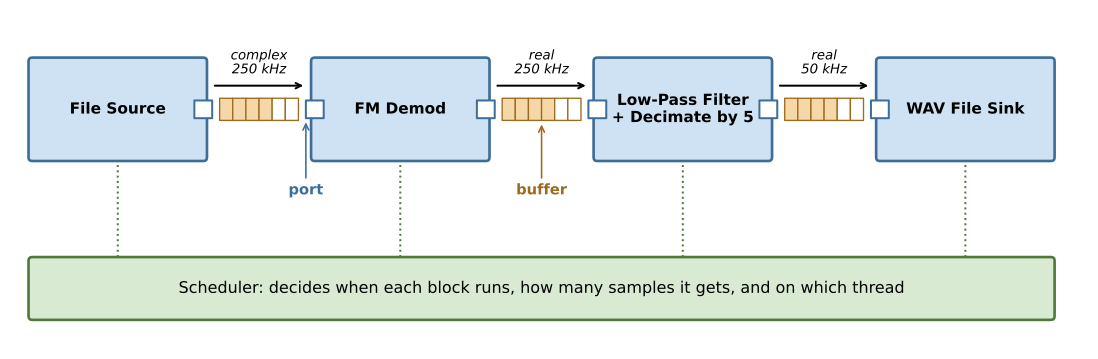
Let’s walk through the parts:

• Blocks are the blue boxes. Each one does a single job, like FM demodulation or filtering, and is written once and reused. Most SDR frameworks ship with hundreds of blocks covering basic signal processing and DSP operations.
• Ports are the connection points on each block. A port has a data type (e.g., a stream of samples, either complex floats or real floats), and the framework checks that you only connect compatible ports, which catches a whole class of bugs before you even run anything.
• Buffers sit between blocks and hold samples that one block has produced but the next block hasn’t consumed yet. Note how the sample rate changes along the chain: 250 kHz complex, then 250 kHz real after the demod, then 50 kHz after decimation. The framework keeps track of these rate changes so each block gets the right number of samples.
• The scheduler decides when each block runs, how many samples it gets to process at a time, and on which thread. If the WAV sink falls behind, the buffer in front of it fills up, and the scheduler stops calling the upstream blocks until there is room again. This is called back-pressure, and it’s what keeps a fast source from overrunning a slow consumer.

On top of these core pieces, most frameworks add a library of blocks, sources and sinks for popular SDR hardware, GUI widgets for plotting, and some way to describe the graph, either graphically (dragging blocks around and drawing wires) or in code. Graphically describing it typically involves a block diagram referred to as a “flowgraph”. Some frameworks also provide a way to attach metadata to specific samples and/or to pass asynchronous messages between blocks (e.g., to change a block’s parameter).

It is easy to confuse SDR frameworks with other kinds of SDR software, because many of these projects blur the lines. The table below is a rough guide:

Category	What it is	Examples
DSP library	Functions you call from your own code, with no scheduler or graph	NumPy/SciPy, liquid-dsp, VOLK, FFTW
Hardware API	Code that gets samples to and from a specific SDR (or many SDRs)	UHD, libiio, SoapySDR, librtlsdr
SDR framework	A runtime that executes a graph of reusable blocks	GNU Radio, REDHAWK, OpenCPI
Application	A finished program for a specific job, possibly with plugins	SDR++, GQRX, SDRangel, SDR#
Protocol stack	A complete implementation of one wireless standard	srsRAN, OpenAirInterface, GNSS-SDR

Note that these layers stack on top of each other. A framework typically uses DSP libraries inside its blocks and hardware APIs inside its source/sink blocks, and some applications and protocol stacks are built on top of a framework (GNSS-SDR, for example, is built on GNU Radio).

It’s also worth knowing that some popular SDR applications have plugin systems that let you add your own processing, which can cover some of the same ground as a framework. SDRangel is built around channel plugins (demodulators and modulators) and feature plugins, and SDR++ has a module system for sources, decoders, and other add-ons. The difference is that you are extending a specific application with a fixed structure (typically a waterfall with demodulators attached to it), rather than building an arbitrary flowgraph.

Do You Need a Framework?

Short answer: probably not, and most people working with SDRs don’t use one. If you are analyzing IQ recordings offline, writing a one-off script to test an idea, or controlling an SDR from a larger Python application, a plain script with NumPy is simpler, easier to debug, and has no learning curve beyond the DSP itself. Many fielded RF systems also do all the high-rate processing in an FPGA, with a relatively thin piece of custom C++ on the host that doesn’t benefit much from a framework.

So when is a framework worth it? Here are the main benefits:

• Tested blocks. Costas loops, clock recovery, polyphase resamplers, and channel models are hard to get right. A framework gives you versions that thousands of people have already debugged.
• Streaming infrastructure. Processing an endless stream in chunks, carrying state between chunks, threading, buffers, and back-pressure are all handled for you.
• Performance. Mature frameworks use SIMD-optimized kernels and run each block on its own thread, so a long chain uses many CPU cores without you writing any multithreaded code.
• Hardware abstraction. Swapping a USRP for a PlutoSDR can be as simple as swapping the source block.
• Rapid prototyping. Graphical editors let you build, run, and tweak a receiver in minutes, with sliders and live plots, which is also great for teaching.
• Community. You can reuse other people’s blocks and entire applications, like satellite decoders or LoRa receivers.

And the drawbacks:

• Learning curve. You now have to learn the framework’s concepts (item sizes, sample rate bookkeeping, how the scheduler behaves) on top of the DSP.
• Hidden DSP. A block called “WBFM Receive” works great until it doesn’t, and then you need to dig into someone else’s code to find out why. This is also why PySDR teaches with plain Python: the point is to see the DSP.
• Awkward fit for bursty logic. Frameworks are built around continuous streams, so packet-based protocols, TX/RX turnaround with tight timing, and “do this, then wait for that” logic can feel like fighting the framework.
• Latency. Buffers between blocks add delay, which can matter for real-time protocols.
• Dependencies and churn. Installing a framework (and especially third-party blocks) can be painful, and blocks written for one major version may not work on the next.
• Licensing. Some frameworks are GPL licensed, which matters if you plan to ship a closed-source product.

As a rule of thumb, reach for a framework when you need continuous real-time streaming, when the blocks you need already exist, or when you want a quick interactive prototype. Stick with a plain script for offline analysis, learning, one-off experiments, and anything where you want full control and visibility over every step.

It is no secret that in the era of AI, existing software (applications to a great extent and frameworks to a lesser extent) loses some of its value, due to how rapidly you can create new software that does exactly what you want. Instead of taking an existing open source application and tweaking it, it’s often easier to just create a new one from scratch. Frameworks hold up better; they lose some value in the era of AI but not all of it, especially if you are planning on collaborating with others or showing off what you created.

Example: FM Receiver Without a Framework

To make this concrete, here is our FM receiver written the PySDR way, with nothing but NumPy and SciPy. We will process an IQ recording of FM that can be downloaded here. This FM receiver will be recreated in every framework we discuss in this chapter.

import numpy as np
from scipy.signal import firwin, lfilter
from scipy.io import wavfile

sample_rate = 250e3
x = np.fromfile('fm_rds_250k_1Msamples.iq', dtype=np.complex64)

x = np.angle(x[1:] * np.conj(x[:-1])) # FM demod

# Low-pass filter to keep only the mono audio (0 to 15 kHz), then decimate by 5 to get 50 kHz
taps = firwin(101, 15e3, fs=sample_rate)
x = lfilter(taps, 1.0, x)
x = x[::5]

# Normalize, convert to 16-bit ints, and save as a WAV file
x = x / np.max(np.abs(x))
wavfile.write('fm.wav', int(sample_rate/5), (x * 32767).astype(np.int16))

Because FM puts the audio in the instantaneous frequency, and frequency is the rate of phase change, the output of the FM demod line is the audio. Open fm.wav in any audio player and you should hear about 4 seconds of the station.

With a live SDR you would have to process samples in chunks, carrying the filter state, the previous sample for the demod, and the decimation phase from one chunk to the next, all while a separate thread keeps up with the incoming samples. That’s very doable (the Real-Time GUIs with PyQt chapter builds a real-time app without a framework), but it’s exactly the plumbing a framework handles for you.

GNU Radio

GNU Radio is the oldest and by far the most widely used open source SDR framework. It was started in 2001 by Eric Blossom with funding from John Gilmore, and today it is used by hobbyists and across academia, industry, and defense. It is written in C++ with Python bindings, licensed under GPL-3, and runs on Linux, macOS, and Windows. If someone says “SDR framework” without qualification, they probably mean GNU Radio. Where GNU Radio really shines is its incredible ecosystem, which consists of:

• Software: Third-party blocks, example flowgraphs, SDR/hardware support, as well as contributors to the core code. There are also applications like GNU Radio World that build on GNU Radio and its ecosystem of software.
• Community: People who use it and develop it, and the GNU Radio conferences that double as a way to bring together folks who work in areas related to SDR and RF signal processing, or simply do it as a hobby.
• Education: From high school to graduate level, it’s used to teach and practice RF and DSP concepts without getting bogged down in code.

Full disclosure: I’m one of the leads of the GNU Radio project, so take my enthusiasm with a grain of salt!

GNU Radio’s current stable series is 3.10. Let’s start with how it maps to the concepts from earlier:

• Blocks are C++ or Python classes. The most common kind is a “sync block”, which outputs one sample for every input sample. There are also decimators and interpolators, which change the rate by a fixed ratio.
• The scheduler runs each block in its own thread (the “thread-per-block” scheduler), so a flowgraph with 20 blocks automatically uses many CPU cores.
• Buffers are circular buffers that use a clever trick: the same physical memory is mapped twice, back to back, so a block can always read or write a contiguous chunk without worrying about wrapping around the end of the buffer.
• Stream tags and messages are two extras GNU Radio adds on top of those core concepts. Stream tags are small pieces of metadata attached to a specific sample, which travel through the flowgraph alongside the samples. For example, the source might tag the first sample with the time it was received, and that tag will come out of the far end of the chain still attached to the corresponding sample, even after decimation. Messages are asynchronous, not tied to any sample, and are used for control (e.g., a GUI slider changing a filter’s cutoff frequency) or for passing around packets once you’ve demodulated bits. Messages use a type system called PMTs (polymorphic types) and are sent between blocks through message ports.
• Performance comes largely from VOLK, the Vector-Optimized Library of Kernels, which picks the fastest SIMD implementation of common operations for whatever CPU you are running on.

The part of GNU Radio most people see first is GNU Radio Companion (GRC), a graphical editor where you drag blocks onto a canvas, draw connections, and press play. Behind the scenes GRC generates a Python script, which you can open, read, and run without GRC. This makes GRC a great way to learn the Python API too.

FM Receiver in GNU Radio 3

In GRC, our receiver is four blocks wired in a row: a File Source, a Quadrature Demod, a Low Pass Filter with its decimation set to 5, and a Wav File Sink. Here is the same flowgraph written directly with the Python API, which is essentially what GRC generates for you, minus the boilerplate:

import numpy as np
from gnuradio import gr, blocks, analog, filter

sample_rate = 250e3

tb = gr.top_block()
src = blocks.file_source(gr.sizeof_gr_complex, 'fm_rds_250k_1Msamples.iq', False)
demod = analog.quadrature_demod_cf(sample_rate / (2 * np.pi * 75e3))  # FM demod, scaled so 75 kHz deviation = 1.0
taps = filter.firdes.low_pass(1.0, sample_rate, 15e3, 5e3)  # 15 kHz cutoff, 5 kHz transition width
lpf = filter.fir_filter_fff(5, taps)  # low-pass filter and decimate by 5
snk = blocks.wavfile_sink('fm.wav', 1, int(sample_rate/5), blocks.FORMAT_WAV, blocks.FORMAT_PCM_16, False)

tb.connect(src, demod, lpf, snk)
tb.run()

Run it and you’ll get essentially the same fm.wav as the plain Python version. The line count is about the same too, but a few things are worth noticing:

• The code describes the graph; it doesn’t process anything. Each line creates a block, connect() wires them together in order, and nothing happens until tb.run() hands the graph to the scheduler, which streams the file through in chunks until the File Source runs out of samples.
• The demod uses a gain instead of a normalization. The Quadrature Demod block computes the exact same angle as our np.angle() line, times a gain. In the NumPy version we normalized by the maximum value at the end, but a streaming flowgraph never sees “the end”, so that’s not an option. Instead we use the fact that broadcast FM has a maximum frequency deviation of 75 kHz, and pick the gain so that full deviation maps to 1.0, which is the full-scale value the WAV sink expects.
• The filter is specified by its transition width, not its number of taps. firdes.low_pass() works out how many taps it needs (121 here) to go from passband to stopband within 5 kHz.
• Decimation is a parameter of the filter. fir_filter_fff(5, taps) only computes every 5th output sample, instead of filtering everything and then throwing 80% of it away like our x[::5] did.
• You keep track of sample rates yourself. GNU Radio 3 doesn’t pass the sample rate along the graph, so everything that depends on it (the demod gain, the filter design, and the WAV sink in this case) has to be told what rate it is running at. Get it wrong and the audio plays at the wrong pitch.

To turn this into a live radio, swap the File Source for an SDR source block (e.g., from gr-osmosdr, gr-uhd, or gr-iio) and the Wav File Sink for an Audio Sink; the blocks in between stay the same.

The flowgraph below is the same receiver running in your browser using GNU Radio World, reading the exact same recording. Instead of writing a WAV file it plays the audio through your speakers, and instead of separate demod and filter blocks it uses the WBFM Receive block, which is a hierarchical block (a block made of other blocks) that bundles the quadrature demod, low-pass filter, decimation, and a de-emphasis filter into one. It also resamples from 250 kHz to 240 kHz first, so that decimating by 5 lands on 48 kHz, a rate every sound card supports. Hit run, give it a moment, and you should hear the station.

Bringing Your Own NumPy Code

One of the most useful features for PySDR readers is the Embedded Python Block. In GRC you can add a block whose code lives right inside the flowgraph, and that code is just a Python class with a work() function that receives NumPy arrays. Here’s the general shape of one, which simply multiplies the signal by a constant:

import numpy as np
from gnuradio import gr

class blk(gr.sync_block):
    def __init__(self, gain=1.0):
        gr.sync_block.__init__(self, name='Multiply by Gain', in_sig=[np.complex64], out_sig=[np.complex64])
        self.gain = gain

    def work(self, input_items, output_items):
        output_items[0][:] = input_items[0] * self.gain
        return len(output_items[0])

The work() function gets called over and over by the scheduler, each time with a new chunk of samples in input_items[0], and it must fill output_items[0] and return how many samples it produced. Anything you learned in this textbook that operates on a NumPy array can go inside work(), which means you can prototype a new algorithm in plain Python, then drop it into a GNU Radio flowgraph and let GNU Radio deal with the SDR hardware, the threading, and the GUI. Just remember that if your algorithm has memory (filters, PLLs, etc.), you need to store that state in self so it carries over between calls to work().

The Ecosystem

A big part of GNU Radio’s value is everything built on top of it. Third-party blocks are distributed as out-of-tree (OOT) modules, and there are hundreds of them, including gr-osmosdr (sources/sinks for many SDRs), gr-satellites (decoders for over a hundred satellites), and gr-lora_sdr (a LoRa transceiver). The CGRAN website catalogs many of them. The easiest way to install GNU Radio along with a bunch of SDR drivers on any OS is radioconda.

You have actually been using GNU Radio throughout this textbook already. The interactive flowgraphs embedded in chapters such as Filters and Synchronization are real GNU Radio, compiled to run inside your browser using GNU Radio World, with no install required.

GNU Radio 4.0

GNU Radio 4.0 (a.k.a. GR4) is a ground-up rewrite of the runtime, and as of this writing it has reached the release-candidate stage (RC3 was released in September 2026), while GNU Radio 3 remains the stable series for production use. The motivation is that GNU Radio 3’s design dates back to the early 2000s, and a lot has changed since then in C++ and in computer hardware. The biggest changes are:

• Much faster. GR4 lets you optionally merge blocks together at compile time, so the buffer between them disappears entirely, along with the trip through memory and the scheduler overhead it costs. The scheduler itself can be swapped out for a custom one.
• Modern C++23. Blocks are written in a much more compact style, and much of the work of connecting blocks is checked at compile time. There’s less boilerplate when writing a custom block, and a block’s logic is no longer spread across a bunch of files.
• Block registry and plugins. GR4’s new registry and plugin system means block metadata (parameters, ports, constraints) can be read programmatically, so blocks can be auto-discovered, UIs generated automatically, and configurations validated. The registry is used for run-time discovery of blocks contained in shared library plugins.

FM Receiver in GNU Radio 4.0

Here is our FM receiver in GR4, written in C++. It was tested against 4.0.0-RC3, and since GR4 is still at the release-candidate stage, expect some of the names to shift before the final release.

#include <gnuradio-4.0/Graph.hpp>
#include <gnuradio-4.0/Scheduler.hpp>
#include <gnuradio-4.0/fileio/BasicFileIo.hpp>
#include <gnuradio-4.0/fileio/WavBlocks.hpp>
#include <gnuradio-4.0/analog/QuadratureDemod.hpp>
#include <gnuradio-4.0/filter/FirDecimator.hpp>
#include <numbers>

int main() {
    using namespace gr;
    const float sample_rate = 250e3f;

    Graph fg;
    auto& src = fg.emplaceBlock<blocks::fileio::BasicFileSource<std::complex<float>>>({{"file_name", std::string("./fm_rds_250k_1Msamples.iq")}});
    auto& demod = fg.emplaceBlock<incubator::analog::QuadratureDemod<float>>({{"gain", sample_rate / (2 * std::numbers::pi * 75e3)}});
    auto& lpf = fg.emplaceBlock<incubator::filter::FirDecimator<float>>({{"decim", 5U}, {"sample_rate", sample_rate}, {"f_low", 15e3f}, {"transition_width", 5e3f}});
    auto& snk = fg.emplaceBlock<blocks::fileio::WavSink<float>>({{"uri", std::string("./fm.wav")}, {"sample_rate", sample_rate / 5}});

    fg.connect<"out", "in">(src, demod).value();
    fg.connect<"out", "in">(demod, lpf).value();
    fg.connect<"out", "in">(lpf, snk).value();

    scheduler::Simple sched;
    sched.exchange(std::move(fg)).value();
    sched.runAndWait().value();
}

The shape is the same as the GNU Radio 3 version: create the blocks, connect them, hand the graph to a scheduler, and run.

FutureSDR

FutureSDR is an SDR framework written in Rust, started in 2021 by Bastian Bloessl (who also wrote the popular GNU Radio WiFi and ZigBee transceivers). It’s licensed under Apache 2.0 and is under active development, with version 0.9 released in October 2026. It is still considered experimental, and its block library is much smaller than GNU Radio’s.

So why build another framework? FutureSDR is designed around a few ideas that are hard to retrofit into an older framework:

• Rust. Rust gives C++-like performance with memory safety guaranteed at compile time, which eliminates whole categories of crashes and race conditions in multithreaded code.
• Async runtime. Instead of one OS thread per block, blocks are async tasks executed by a small pool of worker threads. Schedulers are pluggable, so the same flowgraph can be run with different scheduling strategies depending on whether you care about throughput or latency.
• Runs anywhere, including the browser. FutureSDR compiles to WebAssembly (WASM), so an entire receiver can run inside a web page. It also runs on Linux, Windows, macOS, and Android.
• Accelerators. It was designed from the start with custom buffers that let blocks run on GPUs (through WGPU, which works both natively and in the browser) and FPGAs (e.g., via DMA on Xilinx Zynq), treating them as first-class parts of the flowgraph instead of add-ons.
• Remote control. Every running flowgraph exposes a REST API, so you can inspect it and control it from a web GUI or another program.

FM Receiver in FutureSDR

Here is our receiver in FutureSDR 0.9. Note that FutureSDR uses some unstable Rust features, so you need the nightly Rust compiler (rustup toolchain install nightly) and the audio feature enabled in Cargo.toml for the WAV sink.

use futuresdr::blocks::audio::WavSink;
use futuresdr::blocks::{Apply, FileSource, FirBuilder};
use futuresdr::futuredsp::{firdes, windows};
use futuresdr::hound;
use futuresdr::prelude::*;

fn main() -> Result<()> {
    let sample_rate = 250e3;
    let mut fg = Flowgraph::new();

    let src = FileSource::<Complex32>::new("fm_rds_250k_1Msamples.iq", false);

    // FM demod, which needs to remember the previous sample
    let gain = (sample_rate / (2.0 * std::f64::consts::PI * 75e3)) as f32;
    let mut last = Complex32::new(0.0, 0.0);
    let demod = Apply::new(move |x: &Complex32| -> f32 {
        let y = (x * last.conj()).arg() * gain;
        last = *x;
        y
    });

    // Low-pass filter to keep only the mono audio (0 to 15 kHz), then decimate by 5 to get 50 kHz
    let taps = firdes::lowpass::<f32>(15e3 / sample_rate, &windows::hamming(101, false));
    let lpf = FirBuilder::decimating_with_taps::<f32, f32, _>(5, taps);

    let spec = hound::WavSpec {
        channels: 1,
        sample_rate: (sample_rate / 5.0) as u32,
        bits_per_sample: 32,
        sample_format: hound::SampleFormat::Float,
    };
    let snk = WavSink::<f32>::new("fm.wav", spec);

    connect!(fg, src > demod > lpf > snk);
    Runtime::new().run(fg)?;
    Ok(())
}

REDHAWK, OpenCPI, and the SCA

The frameworks so far grew out of the open source and academic communities. There is a second family of frameworks that came out of the U.S. defense world, and they look quite different, because they were designed to solve a different problem.

The Software Communications Architecture

In the late 1990s the U.S. military launched the Joint Tactical Radio System (JTRS) program, aiming to replace a large number of incompatible military radios with a family of software-defined radios. The central idea was waveform portability: a waveform (the military term for a complete signal processing application, like a specific communications protocol) should be written once and run on radios from different manufacturers. To make that possible, JTRS created the Software Communications Architecture (SCA), whose first version appeared in 2000.

The SCA is not a DSP library; it’s a specification for how software components get described, deployed, connected, configured, and started on a radio’s processors. Components are described in XML files, they communicate over CORBA (a middleware standard for calling functions on objects in other processes or on other machines, which was mandatory up through SCA 2.2.2 and became optional in SCA 4), and a “core framework” on each radio reads those XML files to launch the waveform on whatever processors are available. Notice the emphasis: deployment and portability come first, and the DSP itself is up to you. Several commercial SCA implementations exist, and the specification is still maintained, but it is mostly confined to the military radio world.

REDHAWK

REDHAWK is an SDR framework developed with U.S. government funding, originally for use within the government, and later released as open source (primarily under the LGPL). It borrows heavily from the SCA’s concepts, though it does not try to be SCA compliant, and its focus is on signal processing applications running across a network of ordinary computers rather than on a single tactical radio.

REDHAWK’s vocabulary maps onto the concepts from earlier like this:

• Components are the blocks, written in C++, Python, or Java. Python and Java components each run as their own process, while C++ components (since REDHAWK 2.1) can be loaded together into a single shared process to avoid the overhead of passing samples between processes.
• Waveforms (also called applications) are the flowgraphs, described in XML.
• Devices represent hardware, both SDRs and the computers that components run on, and are managed by device managers.
• A domain manager oversees everything, deciding which computer each component runs on when a waveform is launched, which lets one waveform span several machines.
• An Eclipse-based IDE provides graphical waveform editing and code generation for new components, and there’s a Python “sandbox” for running components interactively.

The killer feature was distribution: you could launch a waveform and have its components spread across a rack of servers, with monitoring and control of everything from one place. The cost is complexity, with lots of XML, CORBA under the hood, and an install that was historically tied to specific versions of Red Hat-family Linux. Development has slowed considerably, with the last release (2.3.2) in early 2023, so REDHAWK is best thought of as a framework you might encounter on an existing government program rather than one you’d pick for a new project.

FM Receiver in REDHAWK

REDHAWK ships with a set of basic components that cover most of our receiver: rh.FileReader reads the IQ file, rh.AmFmPmBasebandDemod performs the FM demod, rh.fastfilter is a low-pass filter (it filters using FFTs, but doesn’t decimate), rh.ArbitraryRateResampler brings the rate down to 50 kHz, and rh.FileWriter saves the result. You would normally drag these onto a canvas in the REDHAWK IDE and draw the connections, and the IDE saves the flowgraph as a waveform described in a “software assembly descriptor” XML file (.sad.xml). The full file is long, so here is an abbreviated version showing the first two components and the first connection:

<softwareassembly id="DCE:..." name="fm_rx">
  <componentfiles>
    <!-- one entry per component type, pointing to that component's .spd.xml file -->
  </componentfiles>
  <partitioning>
    <componentplacement>
      <componentfileref refid="FileReader_..."/>
      <componentinstantiation id="FileReader_1" startorder="0">
        <usagename>FileReader_1</usagename>
        <componentproperties>
          <simpleref refid="source_uri" value="file:///data/fm_rds_250k_1Msamples.iq"/>
          <simpleref refid="file_format" value="COMPLEX_FLOAT_LITTLE_ENDIAN"/>
          <simpleref refid="sample_rate" value="250Ksps"/>
          <simpleref refid="playback_state" value="PLAY"/>
        </componentproperties>
        <findcomponent>
          <namingservice name="FileReader_1"/>
        </findcomponent>
      </componentinstantiation>
    </componentplacement>
    <componentplacement>
      <componentfileref refid="AmFmPmBasebandDemod_..."/>
      <componentinstantiation id="AmFmPmBasebandDemod_1" startorder="1">
        <usagename>AmFmPmBasebandDemod_1</usagename>
        <componentproperties>
          <simpleref refid="freqDeviation" value="75000.0"/>
        </componentproperties>
        <findcomponent>
          <namingservice name="AmFmPmBasebandDemod_1"/>
        </findcomponent>
      </componentinstantiation>
    </componentplacement>
    <!-- fastfilter (lowpass, freq1 = 15000), ArbitraryRateResampler (outputRate = 50000),
         and FileWriter follow the same pattern -->
  </partitioning>
  <assemblycontroller>
    <componentinstantiationref refid="FileReader_1"/>
  </assemblycontroller>
  <connections>
    <connectinterface id="connection_1">
      <usesport>
        <usesidentifier>dataFloat_out</usesidentifier>
        <componentinstantiationref refid="FileReader_1"/>
      </usesport>
      <providesport>
        <providesidentifier>dataFloat_in</providesidentifier>
        <componentinstantiationref refid="AmFmPmBasebandDemod_1"/>
      </providesport>
    </connectinterface>
    <!-- three more connectinterface entries, one per arrow in the flowgraph -->
  </connections>
</softwareassembly>

To run it, you start a domain manager and a device manager, install the waveform into the domain, and launch it from the IDE or from Python. One last wrinkle: rh.FileWriter only writes raw samples or BLUE files (a format common in government signal processing), not WAV, so to listen to the result you would convert the raw float32 file to WAV with a couple of lines of Python. Even abbreviated, this receiver touches far more files than any other version in this chapter, because each component also has its own XML files describing its properties, ports, and implementation. That overhead is the main reason REDHAWK feels heavy for small projects, and it pays off only when you need what it was built for: launching and managing waveforms across many computers.

OpenCPI

OpenCPI (Open Component Portability Infrastructure) is another government-funded, LGPL-3 licensed framework, which dates back to around 2010 and is still actively released (version 2.4.9 came out in 2026). Like REDHAWK, it inherits the SCA’s focus on portable components, but its specialty is heterogeneous systems: a single application can contain components running on a CPU, on an FPGA, and on a GPU, all connected together.

In OpenCPI, components are implemented by workers, and each worker is written in an “authoring model” that matches where it runs: C/C++ for CPUs, VHDL (or Verilog) for FPGAs, and OpenCL for GPUs. The same component can have multiple workers, e.g., a CPU version and an FPGA version, and the framework picks which one to use based on the hardware available when the application is launched. Applications are described in XML, and support for specific hardware platforms (such as Xilinx Zynq-based SDRs) comes from separate platform support projects. This makes OpenCPI attractive for embedded radios where the heavy DSP lives in the FPGA, which, as mentioned earlier, is how many fielded systems are built.

FM Receiver in OpenCPI

OpenCPI’s component library for this kind of work is ocpi.comp.sdr, and it has a floating-point FM demodulator and FIR filter we can use. An OpenCPI application is described in XML (an “OAS”, OpenCPI Application Specification), and it is refreshingly short:

<application done="file_write">
  <instance component="ocpi.core.file_read" connect="frequency_demodulator_xf_f">
    <property name="fileName" value="fm_rds_250k_1Msamples.iq"/>
  </instance>
  <instance component="ocpi.comp.sdr.dsp.frequency_demodulator_xf_f" connect="fir_filter_f"/>
  <instance component="ocpi.comp.sdr.dsp.fir_filter_f" connect="file_write">
    <!-- 64 low-pass taps from firwin(64, 15e3, fs=250e3), as a comma-separated list -->
    <property name="taps" value="..."/>
  </instance>
  <instance component="ocpi.core.file_write">
    <property name="fileName" value="fm_250k.f32"/>
  </instance>
</application>

You run it with ocpirun -v fm_rx.xml, and the done="file_write" attribute tells OpenCPI the application is finished once the file writer has received the end of the file. Unlike the other versions, this one skips the decimate-by-5 step, so the output file is still at 250 kHz, and the FM demod has no gain, so you would need to normalize the output when converting it to WAV.

Notice that the application only names components, never workers. When it’s launched, OpenCPI looks at the hardware available and picks an implementation (worker) for each component. Here’s the core of the CPU worker for the FM demod, which is written in C++ using OpenCPI’s RCC (“Resource-Constrained C/C++”) authoring model:

RCCResult run(bool) {
  if (input.opCode() == Complex_float_timed_sampleSample_OPERATION) {
    size_t length = input.sample().data().size();
    const Complex_float_timed_sampleSampleData* inData = input.sample().data().data();
    RCCFloat* outData = output.sample().data().data();
    output.setOpCode(Float_timed_sampleSample_OPERATION);
    output.sample().data().resize(length);
    for (size_t i = 0; i < length; i++) {
      *outData = atan2(lastSample.real * inData->imaginary - lastSample.imaginary * inData->real,
                       lastSample.real * inData->real + lastSample.imaginary * inData->imaginary);
      lastSample = *inData++;
      outData++;
    }
    return RCC_ADVANCE;
  }
  // ... other opcodes (time, sample interval, flush, metadata, etc.) are passed through
}

Why Do These Feel So Different?

If you come from GNU Radio or plain Python, REDHAWK and OpenCPI can feel heavy, and that’s because they optimize for different things. GNU Radio’s main question is “how do I process this stream of samples quickly?”, while the SCA family’s main question is “how do I deploy, configure, and manage this software on hardware I might not know about yet, possibly built by a different contractor?” That second question matters a lot when a program lasts decades and the radios get replaced several times, and much less when you’re one person with a USRP on your desk.

CyberEther

CyberEther is a GPU-accelerated signal processing and visualization tool created by Luigi Cruz in 2021 as a personal project, and is licensed under MIT. It includes a flowgraph editor and real-time plots rendered on the GPU using Vulkan, Metal, or WebGPU, so it runs on Linux, macOS, Windows, mobile devices, and even in the browser through WebAssembly, and it has a remote interface for running on headless machines. It is very actively developed, but note that it is primarily one person’s project, and while it resembles a framework, there isn’t an ecosystem of third-party blocks or a large community of users building on top of it. Its strength is fast, smooth visualization of wideband signals, which is an area where older frameworks have historically struggled.

FM Receiver in CyberEther

CyberEther can read our raw complex64 recording directly with its File Reader block, which defaults to the CF32 data type (complex float32, the same thing as NumPy’s complex64). You normally build flowgraphs by dragging blocks around in the GUI, but they are saved as human-readable YAML files, so here is our receiver in that form, with the GUI layout information removed:

version: 2
title: FM Receiver from Recording
graph:
  - name: file_reader
    module: file_reader
    device: cpu
    runtime: native
    provider: generic
    config:
      filepath: fm_rds_250k_1Msamples.iq
      fileFormat: raw
      dataType: CF32
      batchSize: 12500
      loop: true
  - name: throttle
    module: throttle
    device: cpu
    runtime: native
    provider: generic
    config:
      intervalMs: 50
    input:
      buffer: '${graph.file_reader.output.signal}'
  - name: fm
    module: fm
    device: cpu
    runtime: native
    provider: generic
    config:
      mode: narrow
      sampleRate: 250000
    input:
      signal: '${graph.throttle.output.buffer}'
  - name: audio
    module: audio
    device: cpu
    runtime: native
    provider: generic
    config:
      inSampleRate: 250000
      outSampleRate: 48000
    input:
      buffer: '${graph.fm.output.signal}'
  - name: spectrum_analyzer
    module: spectrum_analyzer
    device: cpu
    runtime: native
    provider: generic
    input:
      buffer: '${graph.throttle.output.buffer}'

This one is structured a little differently from the others. CyberEther is built around watching and listening to signals live, so the natural sink is the Audio block, which also takes care of resampling the 250 kHz demod output down to the 48 kHz the sound card wants.

Comparison

The timeline below shows when each framework first appeared, colored by whether it came from the community or from the defense world. Release years for the government frameworks are approximate, because they were used internally before being publicly released.

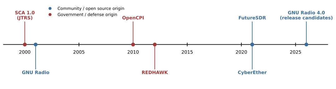
The table below summarizes the frameworks covered in this chapter, as of late 2026.

Framework	Language	License	Status	Graphical Editor	Best For
GNU Radio 3.10	C++, Python	GPL-3	Stable, very active	GRC	General purpose, massive ecosystem
GNU Radio 4.0	C++	MIT	Release candidates	Studio	New projects that can tolerate early adoption
FutureSDR	Rust	Apache 2.0	Active, experimental	Web-based control GUIs	Rust users, browser and accelerator-heavy designs
REDHAWK	C++, Python, Java	LGPL	Unknown; public version is not maintained	Eclipse IDE	Existing government programs, distributed processing
OpenCPI	C++, VHDL	LGPL-3	Active	GUI available	Heterogeneous CPU/FPGA embedded systems
CyberEther	C++	MIT	Active, single developer	Built-in	GPU-accelerated visualization

If you’re just getting started and want to try a framework, GNU Radio 3.X (latest) is the safe choice, simply because of the number of blocks, examples, tutorials, and people who can answer your questions.

External Resources

1. GNU Radio website and tutorials
2. GNU Radio 4 repository
3. GNU Radio World
4. radioconda installer
5. FutureSDR website and repository
6. REDHAWK documentation and repository
7. OpenCPI documentation and repository
8. CyberEther website and repository